4.10.4: Apollo 9
Apollo 8’s hurried conversion to a lunar mission still left some technical issues to be resolved for the Apollo programme. The LM and other important equipment were still untested in a space environment, and docking procedures with it needed to be worked out.
This testing was left to the crew of Apollo 9: Rusty Schweickart, James McDivitt and David Scott (the only one of the three to make it to the moon). It launched at 16:00 GMT on 03/03/69, landing 10 days later on 13/03/69. The mission timeline can be found here.
The transcripts from the flight can be found here, but to be frank they are possibly the dullest transcripts of any mission. The vast majority of the conversations are technical in nature, and there is little in the way of banter recorded between the crew and Houston (certainly when compared with other missions). On top of that, neither the weather nor photography are discussed in any great detail other than requests from the ground to photograph specific targets, and little confirmation is given that these have actually been taken (although they clearly were).
The images that were taken during the mission can be found, as usual, at the Apollo Image Atlas, and high quality TIFF scans can also be found at archive.org by searching for Apollo 9. In total 1373 photographs were exposed on 11 magazines, although a substantial amount of these are from a bank of 4 cameras comprising the Lunar Multispectral Experiment (see here for more details). Detailed information about the content and location of photographs can be found in this report and accompanying spreadsheet, and for the Multispectral photos, here.
In addition to still images, video images were recorded and much of this can be found in various sources in the internet, but perhaps the best are here and here, which includes some of the most stunning sequences taken from an orbiting craft, particularly the shots taken of the CSM from the LM. Footage taken from the CSM of the LM was the inspiration for this section and will be discussed at length later.
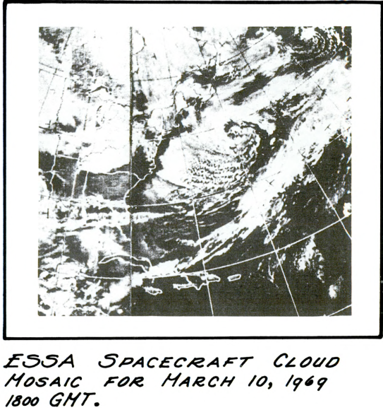
The best satellite source is the ESSA data catalogue, which can be found here, although ATS data are also available here. NIMBUS data would be available, but the quality is generally so poor there is little point in using it. Additional sources include this image of tropical storm Rita from 08/03/69, a brief mention of Apollo 9 imagery in this journal article AMS, and an ESSA image from March 7th is given in this article studying Brazilian weather. Another ESSA image for March 10th can be found here.
As with a lunar mission, one of the first tasks to be undertaken on an Apollo mission is the extraction of the LM from the SIV-
AS09-
Figure 4.10.58: GAP scan of AS09-
What the photograph shows is a relatively cloud free ocean off the coast, a large mass of thin cloud in the north of the USA, some coastal cloud on the north Mexican shoreline and a cloud free area over Mexico and the southern USA. This would seem to be what the satellite image shows us, within the limitations identified in earlier discussions of these orbital missions. On the ESSA image dated the 4th, the cloud is much less clear and is much further inland, and on the day before launch this area was completely clear.
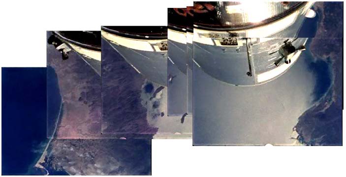
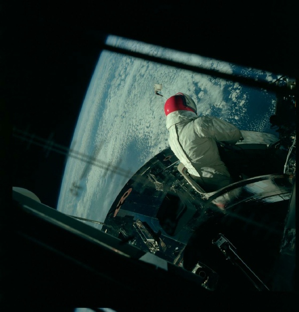
The next major stage in the mission was the EVA carried out by the crew, which involved Scott emerging from the CSM while LM pilot Schweickart observed from a loftier position out of the LM hatch as he tested out the PLSS equipment. They practised a variety of simple procedures, all of which were filmed and photographed from several angles, the most spectacular being from the 100 mile up viewpoint of the LMP.
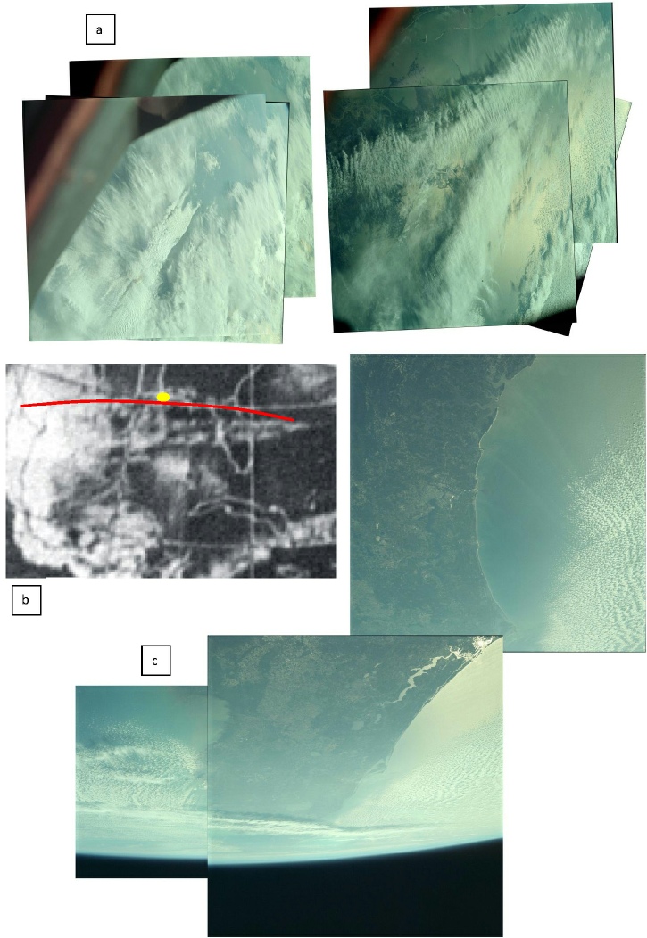
While the photographs are stunning, the best way to determine where they were geographically is by looking at the video footage, which is effectively in three segments separated by brief pauses in filming: one over the Pacific ocean, one crossing the Gulf of California and the final part crossing the southern US/Mexican border area and ending north of Galveston with the Mexican Gulf below.
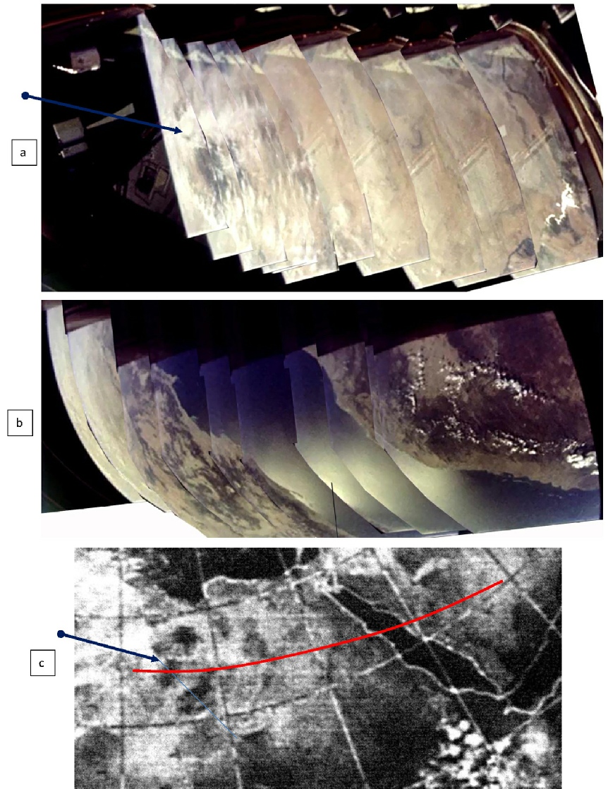
To illustrate this, screenshots of the video have been taken at regular intervals and overlapped to form a continuous image. The results are given in figure 4.10.59a-
Figure 4.10.60 shows the ESSA image covering the same area from 06/03/69.
a) Pacific Footage
b) Baja California
c) Texas
Figure 4.10.59: Screengrabs from Apollo 9 video footage of the EVA compiled into continuous images.
It is difficult to pinpoint with certainty the location of the first section of video footage. It is evidently over a long expanse of ocean, and we know it must be the Pacific because it occurs before the Baja California segment.
The EVA started at 16:59 on 06/03/69 with the opening of the LM hatch, followed a few minutes later by the opening of the CM hatch. As the foot of the LMP emerged from the hatch, the signal was being routed through Huntsville, a ship stationed east of Papua New Guinea, and shortly after the commander emerged they switched to Redstone, stationed at roughly the start of the red line in figure 4.10.60. It seems reasonable to assume then, that figure 4.10.59a shows the EVA passing over the light cloud west of Baja California, finally passing over clear blue ocean just off the coast.
The cloud free zone continues all the way across Mexico and the southern USA, and it is possible to make out Lago Boquilla, Lake Amistad and Canyon Lake on the way to the last section at Galveston, where some beautiful cloud formations can be seen stretching into the Gulf before a much more solid band of cloud is seen in the distance over Florida.
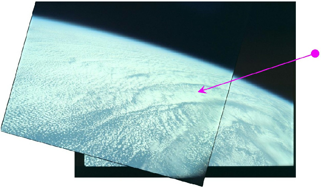
At the end of the video sequence, there is a bit of rapid camera work while passing over the large bank of cloud covering the eastern Gulf coast, before a good shot is obtained that looks eastwards. This is shown in figure 4.10.61, and the patterns in the cloud suggest that the shot is taken looking south-
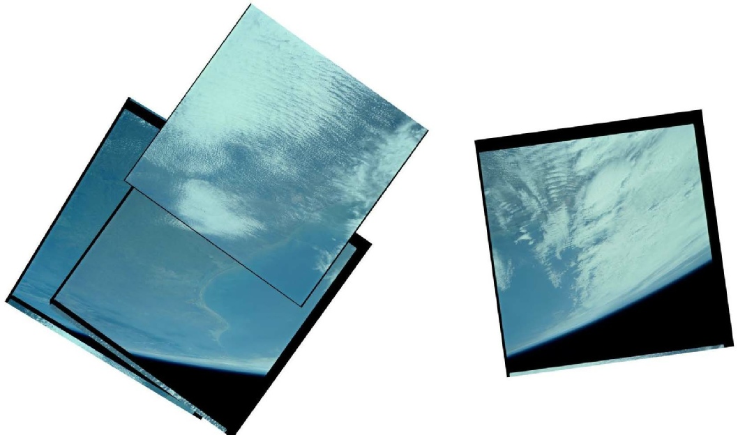
In addition to the video footage, there are still images of the Gulf portion of the EVA taken by Schweickart, and these can be joined together to form the photomontage in figure 4.10.62. The photography report for the mission actually mis-
There are also still images of the Pacific sequence of the video taken by the LMP to be found on magazine 20, and these seem to be taken above the location of Redstone, looking westwards. Figure 4.10.63 shows one of these photographs, AS09-
Figure 4.10.63: GAP scan of AS09-
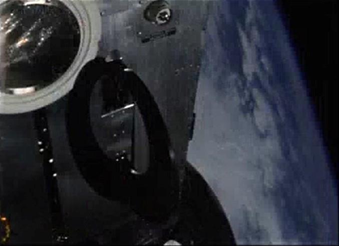
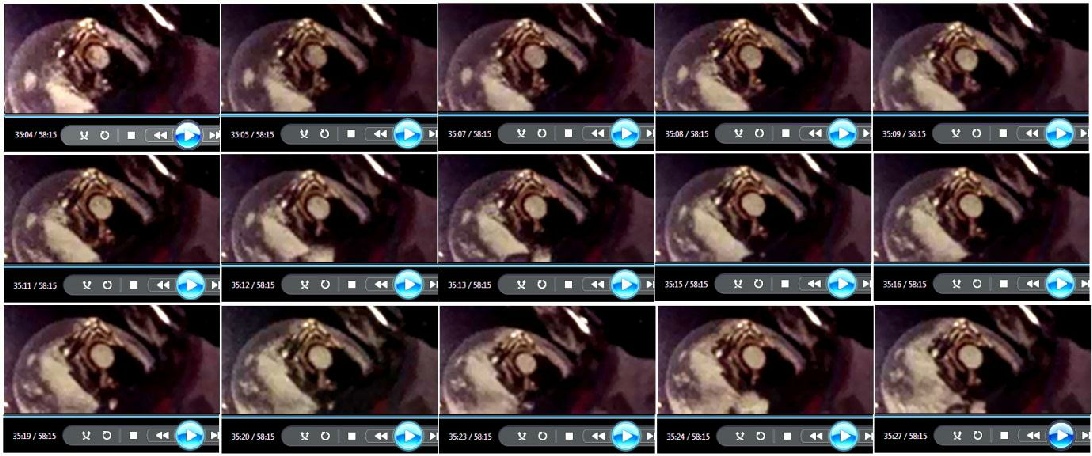
There is another view of the EVA featuring the weather beneath Apollo , but it is not perhaps where you would expect to find it. One of the cameras used to film the EVA was attached to the CM hatch window – it can be seen in figure 4.10.64.
Figure 4.10.64: Close-
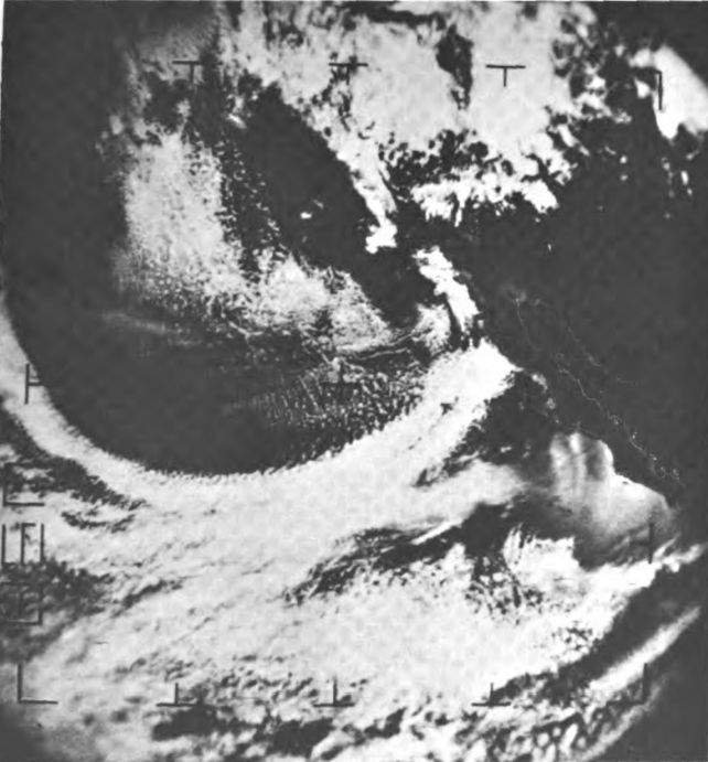
In the video footage shot by this camera there are several moments when Schweickart is directly in front of it. Reflected in his helmet is the view below him: Earth. Figure 4.40.65 shows a collection of screenshots taken of Schweickart in this sequence. The screenshots have been reversed, because the helmet is reflecting the image below and is therefore showing it back to front, but the time markers have been left as in the original screenshot.
It should be emphasised that the curvature visible is obviously a product of the helmet, and is not the actual curvature of the Earth below. It isn’t clear what weather systems the footage is showing, and as Schweickart is mostly out of shot during the video it is difficult to tie it down to his actions, but as the continental landmass is mostly clear it can only be over the Pacific or from the Mexican gulf. If a choice had to be made, it is possible that the large isolated ‘blob’ of cloud in the top left image is the same one visible on the eastern side of figure 4.10.62, just inland of the Gulf coast.
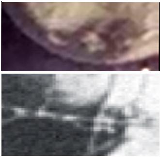
It is also interesting to compare a rotated view of the last image with a section of the ESSA mosaic showing the coastlines of Louisiana and Mississippi (figure 4.10.66).
What is obvious is that Schweickart is looking at a moving scene beneath him, and that the scene is the terrestrial weather. Similar views are to be had in Scott’s helmet eg AS09-
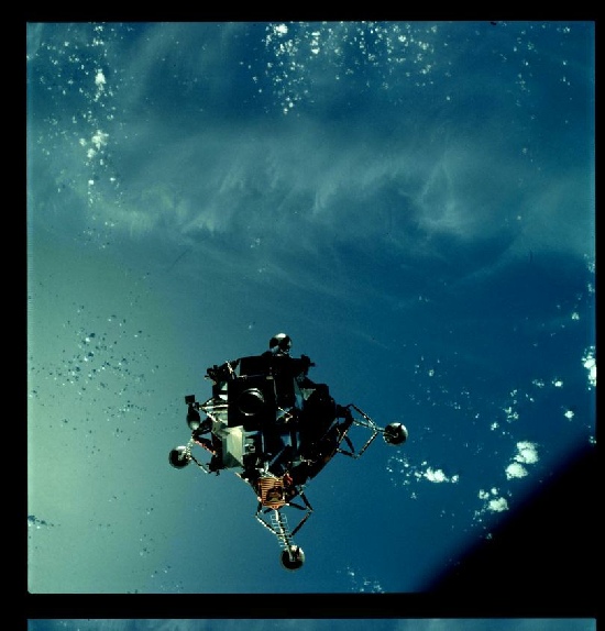
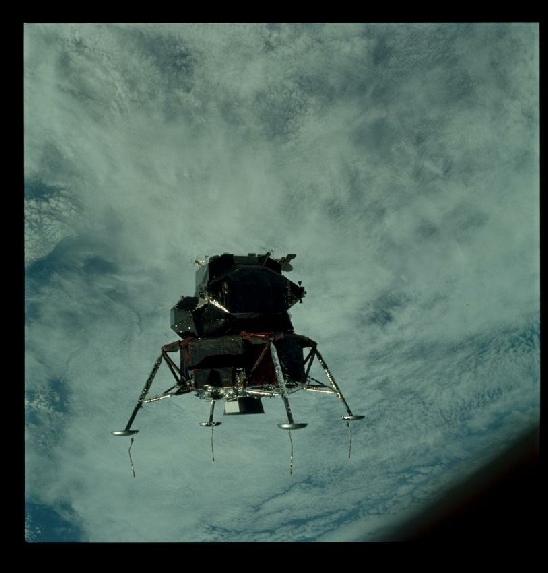
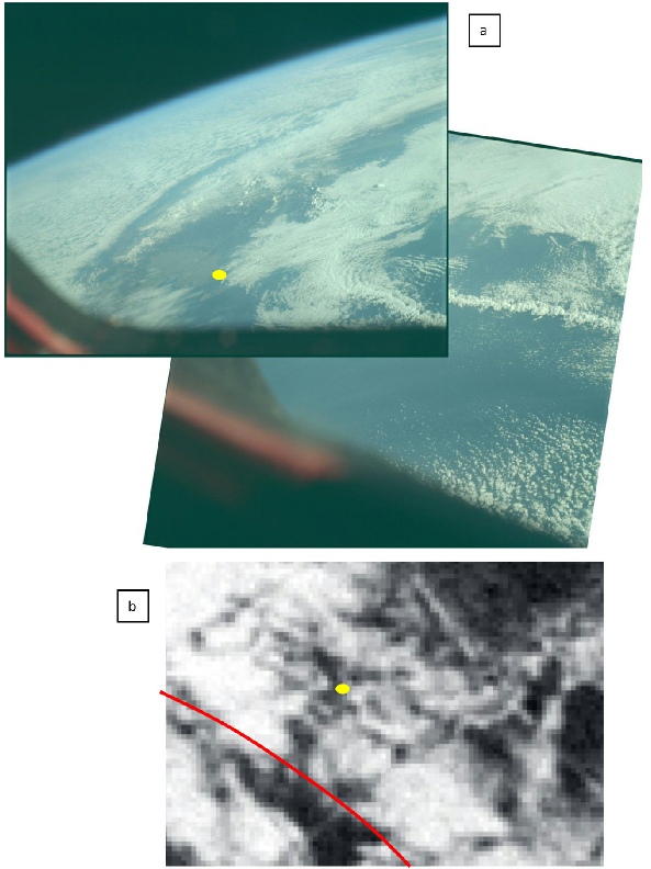
The next step in the mission was to test the LM in solo flight, and therein lies the subject of the challenge that led to the writing of this section. The challenge was: identify the location of the two photographs in figure 4.10.67, and the assumption of the challenger was that it would not be possible. His was the claim that Apollo 9 was faked and did not occur, and he was confident that he would be able to continue to claim so when the location of the image proved impossible.
This author likes a challenge.
The solution to the problem of locating these images is, however, a simple one of logical deduction using all of the information available – something conspiracy theorists are not famed for doing.
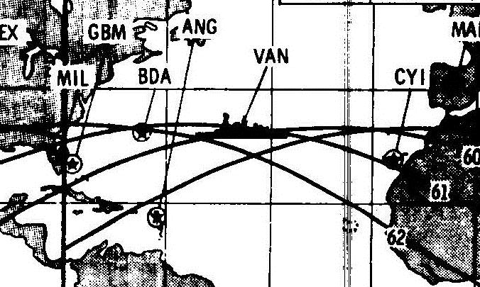
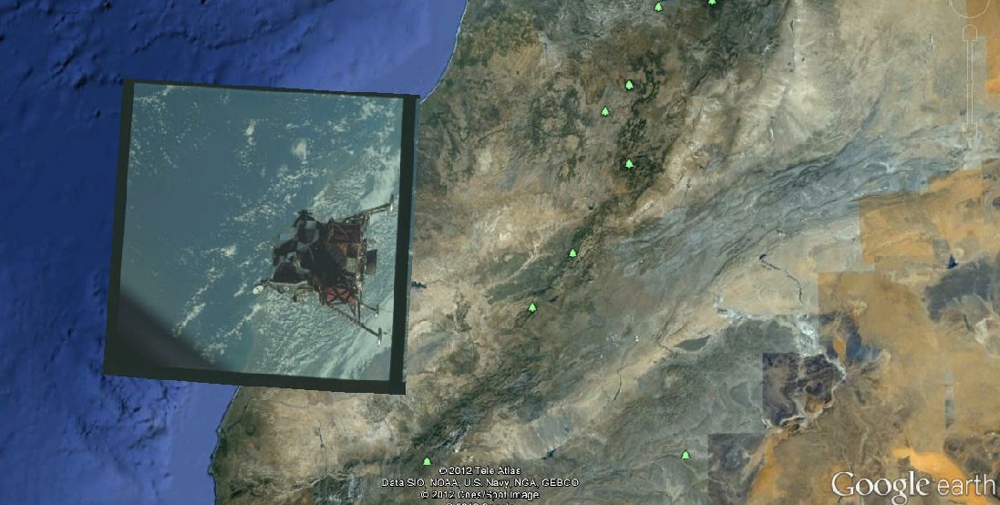
The undocking of Gumdrop and Spider took place at 12:39 07/03/69, 92 hours and 39 minutes in to the mission. At this point, the communications were being routed through Antigua. The orbital path of the two craft at that point follows one across the Atlantic and hitting the coast around Morocco, as shown in figure 4.1068.
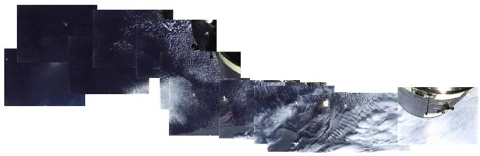
In order to solve the mystery of where these two images are in that Atlantic path, we need to switch to the video footage of the ‘formation flying’ of the two vessels. As before, it is possible to take regular screenshots and merge them together to get a continuous transect of the Atlantic ocean.
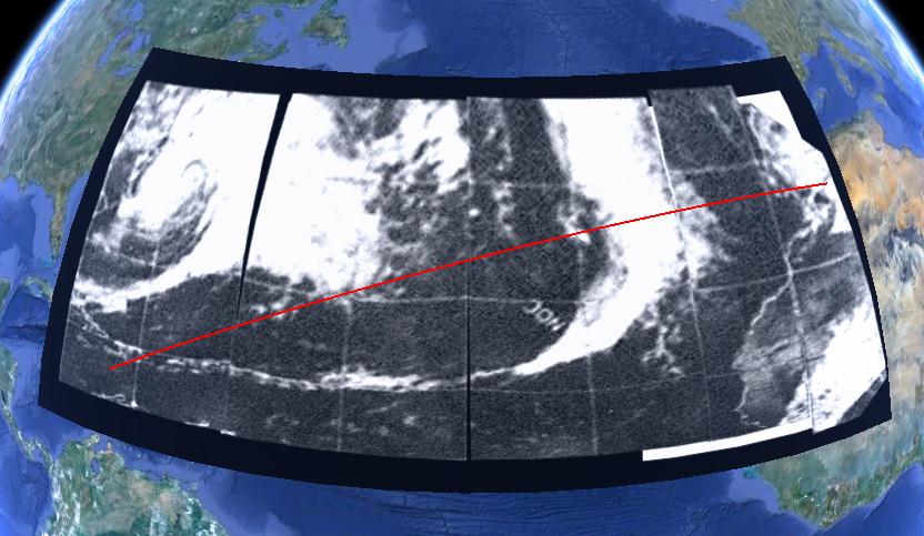
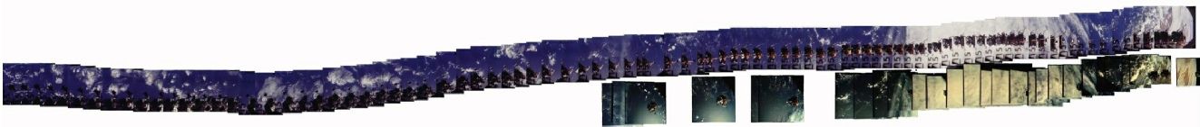
As we know that the event occurred on 07/03/69, and we know where, we can say with certainty that the ESSA 7 mosaic from that date covering the north Atlantic is the correct one to use. In order to make life easier, it is possible to superimpose that mosaic on a Google Earth sphere, as this will allow us to compare the video montage. This is shown below in figure 4.10.69, and the montage itself in figure 4.10.70, in which the photographs taken during the formation flying have been placed according to their position in the video montage.
Figure 4.10.69: ESSA photomosaic from 07/03/69 superimposed on Google Earth. The red line indicates the Apollo 9 flight path.
Figure 4.10.70: Photomosaic of Apollo 9 LM formation flying with photographs from magazine 21 in their geographically correct location. Click here for a much larger version of the photomosaic only.
As figure 4.10.70 shows, the photographs clearly match up with the weather patterns on the video footage, but can we be certain that we have the locations correct?.
The best clue here comes near the end of the sequence in the form of AS09-
Figure 4.10.71: AS09-
So, we have the start of the formation flying as somewhere in the Caribbean, and the end of it over Morocco. Does this now allow us to pinpoint the location of the two photographs? The answer is in figure 4.10.72, and, to put it bluntly, the answer is ‘yes’.
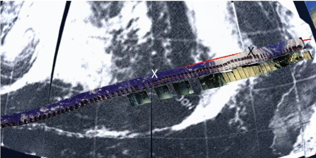
Figure 4.10.72: Photomontage from video footage of ‘formation flying’ matched with photographs from magazine 21, and superimposed on ESSA photomosaic from 07/03/69.
The overlay is not perfect, but considering that the ESSA mosaic superimposed on Google Earth has been perspective distorted, and there has been no attempt at correcting the orientation of the video stills, there is an excellent match between the clouds shown and the video photomontage. Even the length of the video sequence matches the distance that would be covered – just over 4000 miles in about 15 minutes where the ocean is visible on the video.
The still images are placed in their correct position underneath the video montage, and this allows us to state with a good degree of certainty that AS09-
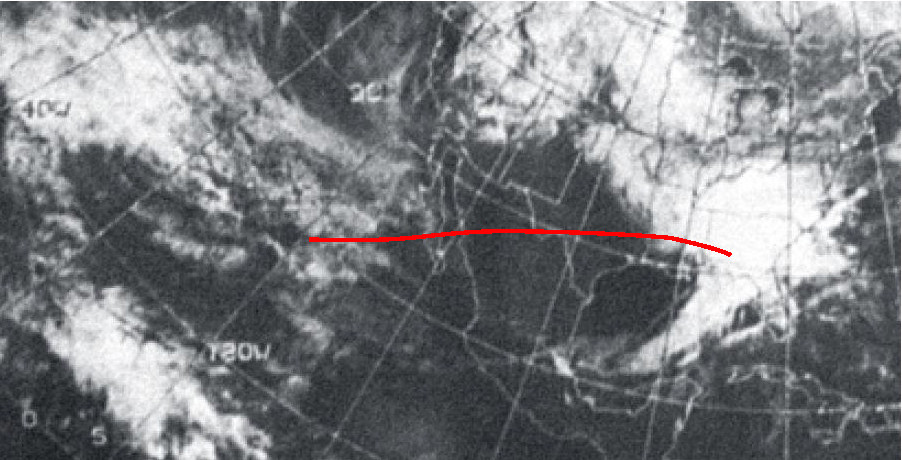
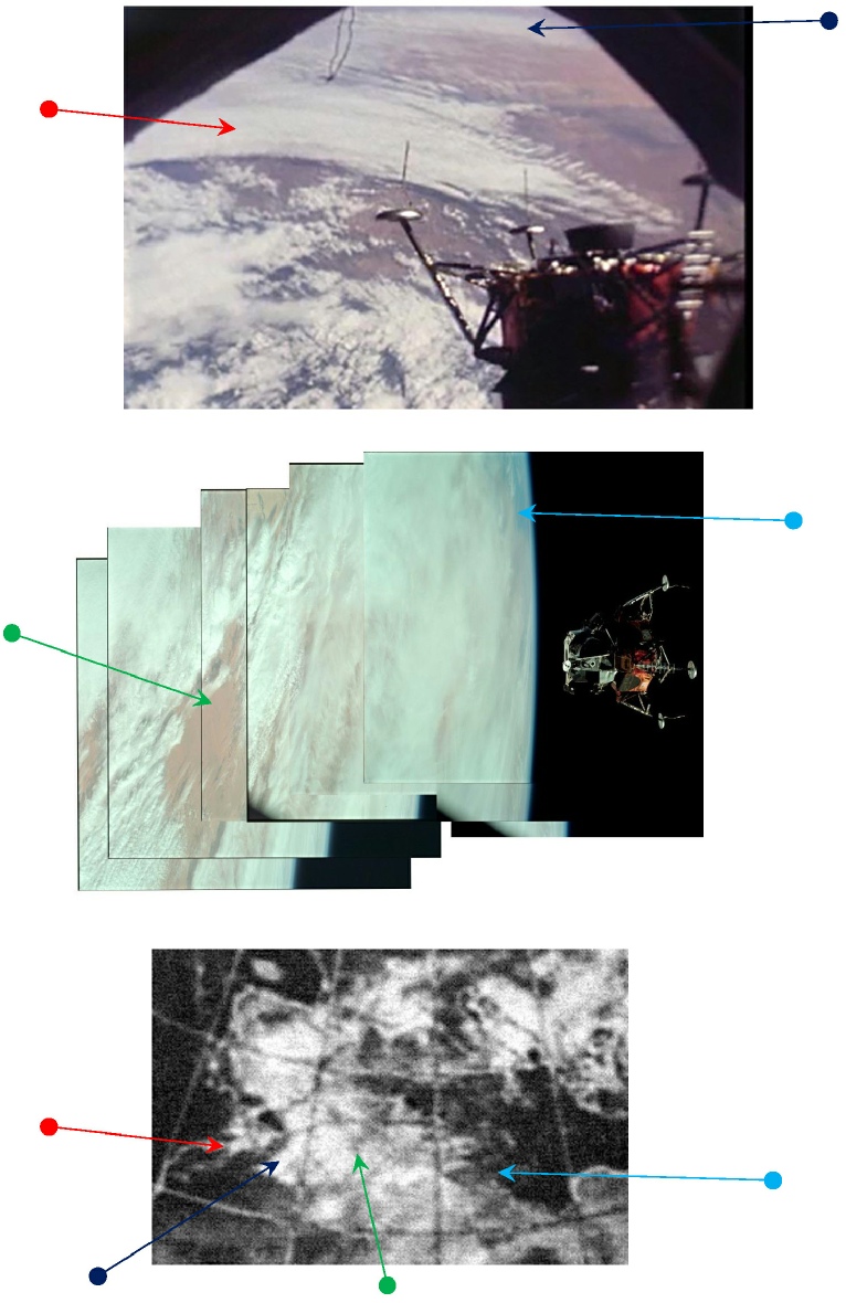
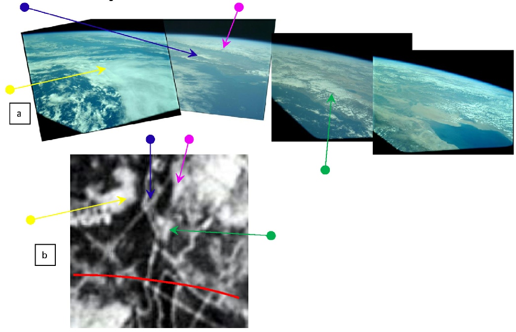
The end of the video sees the camera view move to a more oblique view, and that view can also be seen in the series of photographs beyond the Moroccan coast, where the vista extends as far as Libya. There is, on that view, a clear shot of cloud formations that ought to be visible on the satellite data. Figure 4.10.73a-
Figure 4.10.73: Annotated views of north Africa: a) From video footage (top) b) Photomontage of AS09-
The bank of cloud found in the video still is also very obvious in the ESSA image, which was taken a couple of hours after Apollo 9’s images. Further inland there is the patchy area of cloud that I have identified with a green arrow on the still image montage. This is a more approximate location on the ESSA photograph than the others used, but it fits with the other features visible, most obviously the location of the Tunisian and Libyan coast in the distance.
We can also be certain that we have the correct date for these cloud features, as figure 4.10.73 shows that the cloud features were not the same on the days before or after the formation flying sequence.
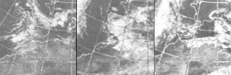
Figure 4.10.74: ESSA images from the 6th (left) 7th (centre) and 8th (right) of March 1969.
Could there have been some magical jiggery-
It is a shame that the person who made the original challenge leading to the preceding analysis was banned from the forum in which it was made shortly before the response to it was posted. He may never have seen his argument comprehensively refuted, and he might still be ignorant of the facts presented. No sleep has been lost over this.
After a few more orbits, the LM descent stage was jettisoned, and there was more formation flying of the LM ascent stage and CSM. Separation of the LM into its component parts occurred at 96:16 MET, or 16:16 on 07/03/69. Formation flying is recorded as occurring at 18:40, and the LM & CSM were re-
At the time of separation, communications were being routed through Tananarive on the island of Madagascar, although the flight plan records the initiation of the co-
Much of the early co-
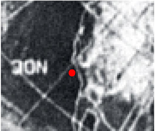
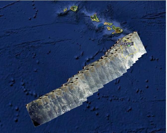
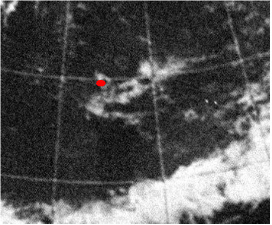
The preceding 10 or so images can be combined to produce a photomontage, but as the camera is quite oblique and the photographs are taken close together, they are little different and not quite as good as a sequence of screenshots from the video footage of the event. That video sequence is shown below, roughly to scale and superimposed on Google Earth in figure 4.10.76, together with the ESSA image of Hawaii (identified by the red dot).
Figure 4.10.76: Photomontage of video screenshots from the ascent stage flight towards Hawaii on 07/03/69
The cloud surrounding Big Island in the ESSA photo also seems to be evident in the video montage in figure 4.10.79, as does the light cloud seen on the approach to the island.
The location of the video sequence prior to that of the Hawaii approach is a little less clear. It consists of a long sequence of ocean shot at varying speed, with no land mass evident. The amount of time involved between the initial co-
The satellite image available for the 7th suggests that the equatorial region between Australia and Hawaii should feature a thick band of cloud bounded by much clearer conditions, but this doesn’t appear to be what the footage shows. It seems more likely that it shows the ocean between Madagascar and western Australia. Figure 4.10.77 shows the video screenshot montage compared with the ESSA mosaics over the Indian Ocean and Pacific respectively.
Figure 4.10.77: Ascent stage flight paths shown by a) video montage (top) b) Australia to Hawaii (bottom left) and c) Madagascar to Australia (bottom right).
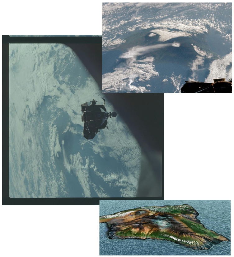
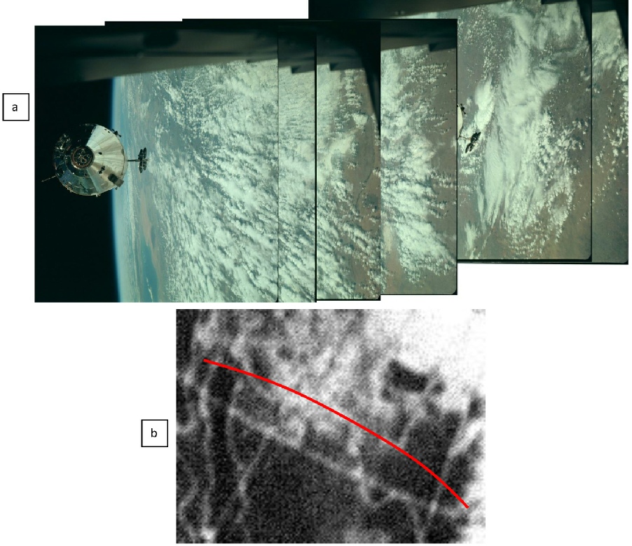
While the LM was being photographed by the command module, the command module was also being photographed and filmed by the LM. There is a particularly impressive film sequence taken (according to the narrative in ‘Three to make ready’, a NASA documentary on the mission) while the descent and ascent stages were still joined together. The start of the sequence looks back eastwards across Egypt (the Nile is visible at one point), and towards the end the Red Sea is shown beautifully as the LM recedes from the CSM. Figure 4.10.78a shows the view back across Egypt towards Libya, and 4.10.78b the view of the Red Sea. Figure 4.10.78c shows the ESSA mosaic of the region on the 7th.
While much of the desert area is cloud free, it is possible to make out the stripes of cloud in the darker patches of the Libyan desert (blue arrow), that would, if you were to go far enough east, eventually lead to the larger cloud patterns featured in images taken from the CSM.
There are also images of the CSM taken after separation of the descent and ascent stages and these are to be found in magazine 24, Several frames that can be joined together to make a longer montage, namely AS09-
Figure 4.10.79 a) Photomontage of the view of the CSM from the ascent stage (top). Note the reflection of the ground and clouds in the CM’s reflective covering. b) ESSA mosaic from 07/03/69 (bottom). Red line indicates approximate orbital path
The video footage of the CSM hovering above the Red Sea is matched only by the still images of the shiny spacecraft above its homeland, aerials pointed towards ground receivers, the clouds reflected in the thin skin separating the human cargo from an icy breathless void.
The thin clouds above New Mexico and Texas are there in the ESSA mosaic just as clearly as the clear skies over the Californian Gulf visible in the distance. While you would be hard pressed to identify specific cloud features in ESSA’s photography, you would be equally hard pressed to deny that the clouds in the photograph are not those pictured by the orbiting satellite.
Once the ascent module was discarded, there are few events that allow us to be completely certain when a photograph was taken other than the records kept by the crew, but there are still several days’ worth of photographic objectives to study!
While the relative low altitude of these missions continues to make comparison with satellite photomosaics difficult, there are several occasions here multiple images can be combined to produce a much broader image that can be used. Two such montages are available from the 8th of March.
The first occurs with views of the Californian coastline, recorded as being taken on the 8th, using AS09-
There is a good degree of correspondence here between the ESSA mosaic and the still image montage, so much so that it is actually worth putting a few arrows on -
Meanwhile, on the opposite coast, a few more photographs were taken looking up the eastern seaboard from South Caroline towards a cloudy New York. The photomosaic of images AS09-
Figure 4.10.81: a) Photomontage of AS09-
This pass by ESSA would have been commenced at 18:06, compared with the recorded time for the Apollo images of 17:16. It is difficult to make out the main cloud features because they are quite small, but suggested locations of the two obvious ones are shown by the green and yellow arrows.
A much easier to place cloud system described as in the Atlantic can be found in images AS09-
Figure 4.10.82: AS09-
The east-
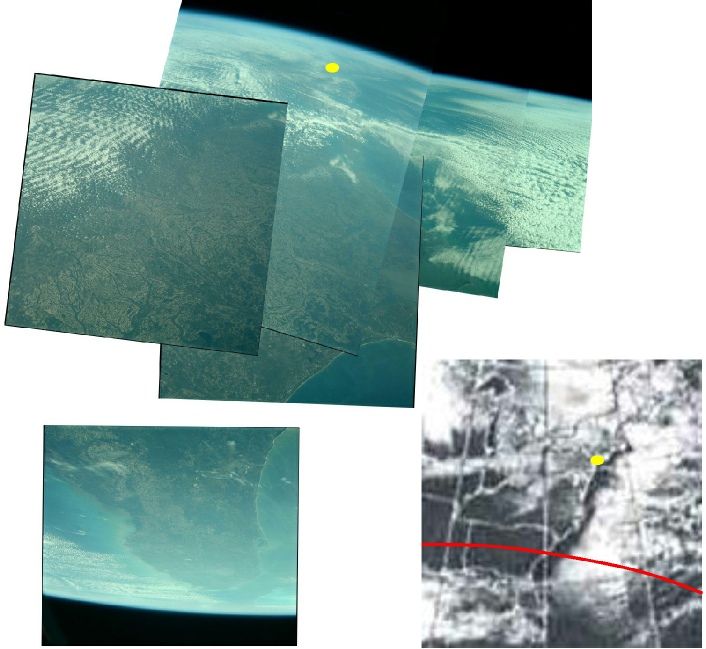
We return to the US on the 10th, with a series of pictures covering the Gulf and Florida area taken around 17:40 GMT. The first set (AS09-
The ESSA pass for this area was commenced at 20:06, so roughly two and a half hours elapse before the Apollo photographs are taken. The spear-
Zooming in on 4.10.86c also shows Cape Kennedy’s launch pads.
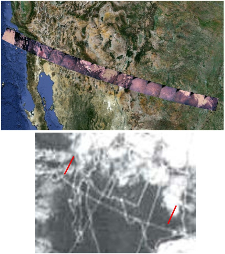
Figure 4.10.83: Above: ESSA image dated 10/03/69 (Source)
Right: a) Photomontage of AS09-
A few hours later, the crew take a couple of photographs of central Honshu, Japan, in the form of AS09-
Figure 4.10.84: a) Photomontage of AS09-
Again the ESSA mosaic lags behind the Apollo photograph by some time (04:06 on the 11th for the former, 23:35 on the 10th for the latter), but there is still a clear area over Nagaya and a bank of cloud behind it. There are also cloud formations nearby that would match the thin strip of cloud in the area.
On the following day we return to the eastern US seaboard with a montage of images AS09-
Figure 4.10.85: a) Photomontage of AS09-
What we can see in the photomontage is clear skies over the southern states, light cloud over the gulf and northern USA merging with thicker cloud off the coast. The ESSA view shows the same scene, with a few minor differences, easily explained by the time difference between the mid-
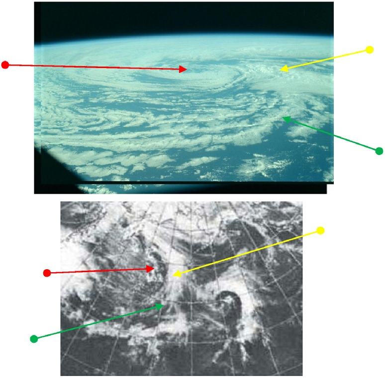
Meanwhile, in the Pacific, a spectacular cyclonic system is captured in AS09-
Figure 4.10.86: a) Photomontage of AS09-
Although there are two cyclonic patterns evident on the ESSA montage, there are a number of features identified with arrows that allow us to be certain that the position given in the photography report is accurate. The time difference between the two sets of images (19:17 on 11/03/68 for the Apollo photographs compared with around 01:01 on 12/03/69 for ESSA) is the main reason that accounts for the differences between the two – notably the much less well defined central whirl of cloud in the ESSA image.
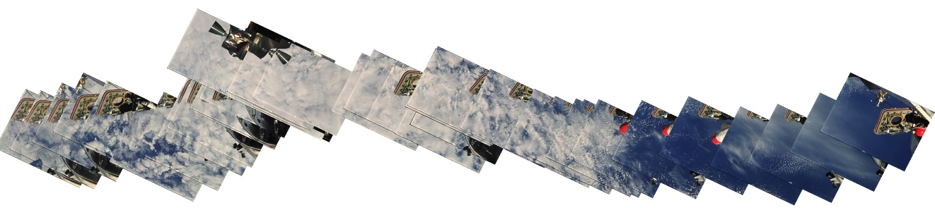
And finally we reach 12/03/69 – the last full day of the mission, and for today’s example we turn to one of the multispectral photography passes that were carried out daily after the completion of the EVA and LM testing part of the mission. On one pass completed on the 12th, successive images were taken making a continuous transect starting from Baja California and ending in Texas. These images (AS09-
The pass starts with a mass of cloud west of the coast, intersects another cloud mass in the central portion, before ending with another small area of cloud. The ESSA mosaic shows exactly the same pattern despite it having been assembled over several hours compared with several minutes for the Apollo photomontage. Apollo’s photographs were commenced at 16:27, compared with ESSA’s 20:06 commencement over that part of north America.
24 hours after commencing this pass over north America, the crew splashed down in the Atlantic, and NASA began preparing for Apollo 10’s full rehearsal for the lunar landings.
4.10.5 Conclusions – again.
So, what have we learned in this section?
It should be obvious from the preceding discussions that LEO missions do not cover anything like enough of the Earth’s surface to show a complete globe. Only when the orbits become highly elliptical or when the camera view is very oblique do we get a significant portion of the Earth’s surface covered (I refer you here to the sections here and here where those claims are also examined).
The well-
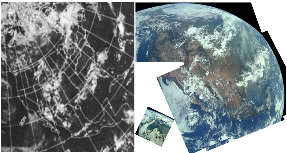
Even a spacecraft positioned a few thousand miles up would not see the entire globe – as shown in the montage in figure 4.10.88. This image is a combination of Apollo 11 made to demonstrate what was being shown by the photographs to sceptics – it seemed a shame to waste it. It is shown with the appropriate ESSA mosaic for reference as well as a mosaic of the latest NIMBUS scans. Also included in the image is an inset of AS11-
Figure 4.10.88: ESSA mosaic from 16/07/69 (left) compared with photomontage of AS11-
Two things should be immediately obvious. Firstly, the amount of the surface visible in the component images of the larger photomontage is vastly greater than the still-
Secondly, there is the change in weather between the two images. Even over just a couple of hours there has been a distinct alteration in the pattern of clouds over Baja California. This again illustrates the general rule when looking at the micro-
Perhaps less obvious is the change in angle of the photographs. The LEO image is looking across the surface towards the horizon, and the elongation of landscape features (and fantastic shadows under the larger clouds) is visible as a result of this. The post-
Given the issues just outlined, can we be confident that we have identified weather systems appropriately in the preceding sections? There is always the danger of pareidolia – seeing what you want to see, and I have always strived to avoid that. Certainly in some of the photographs it is difficult to be absolutely certain, but in others it is much clearer.
What has been demonstrated is that with diligence, detective work and the application of logic, it is possible to determine where photographs have been taken, when, and what they should be showing. While in some cases it hasn’t been possible to be absolutely certain that we have identified a specific cloud, not once has there been an occasion where someone can say ‘this is completely wrong’.
Can we be sure that Apollo 7 & 9 did happen as described?
Yes, of course we can. Only an idiot would claim otherwise. The photographs and video footage are obviously genuine, and techniques that could produce ‘fake’ ones of such accuracy and realism would not exist for decades after the missions (and arguably still don’t).
The only possible motivation for claiming them to be fake is that accepting Apollo 7 and 9’s testing of Apollo’s techniques and hardware seriously compromises claims that astronauts could not have reached,, or survived on, the lunar surface. A working LM and a functional PLSS completely ruins sceptical claims that the equipment was untested and incapable of the jobs required of them.
Apollo deniers need to face facts: we went to the moon in tried and tested equipment and took photographs and films to prove it. Those photographs and films feature Earth, and that Earth looks different every day. Every satellite photograph is a visual fingerprint uniquely identifying a moment in time, and those fingerprints match Apollo’s visual record consistently and accurately.


 Back to Mission Index
Back to CATM Index
Back to Apollo Index
Next Section
Previous Section
Back to Mission Index
Back to CATM Index
Back to Apollo Index
Next Section
Previous Section
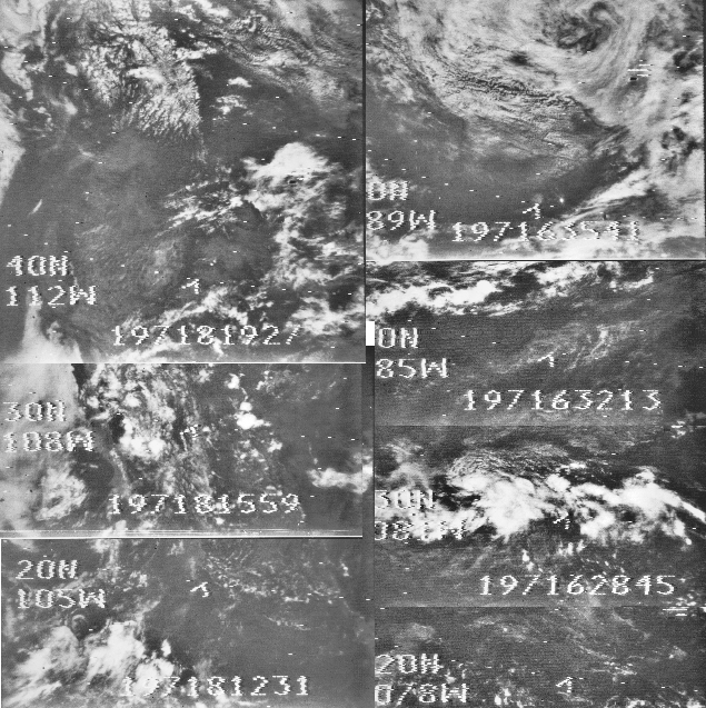
Figure 4.10.80: a) Photomontage of AS09-
Figure 4.10.60: ESSA image dated 06/03/68. Approximate path of Apollo 9 shown in red (Above).
Left: ESSA 8 tile showing the Baja California area (Source).
Figure 4.10.61: View at the end of the EVA video sequence.
Figure 4.10.62: Photomontage of GAP scans of AS09-
Figure 4.10.65: Succession of reversed screenshots from video taken by the CM window camera during the Apollo 9 EVA.
Figure 4.10.66: Helmet reflection (top) compared with ESSA view (bottom)
Figure 4.10.67: GAP scans of AS09-
Figure 4.10.68: Flight paths across the Atlantic for Apollo 9. Source: NASA
Figure 4.10.75: AS09-
Figure 4.10.78: North Africa as seen from the LM a) Looking west towards Egypt and Libya (top) b) Over the Red Sea (middle) and c) The ESSA mosaic from 07/03/69 – red line indicates orbital path
Figure 4.10.87: a) Photomontage of AS09-