Chandrayaan
Chandrayaan data are difficult to deal with, but there is plenty of it and it can be very detailed indeed. Like China’s website their servers are somewhat unreliable and slow, which means that the files can also be difficult to deal with. This site describes how they got hold of data and played around with it, and I’ll give my own version.
There are two sets of data we can play with here, the Terrain Mapping Camera (TMC) and the Digital Elevation Models (DEM) built from those observations. We’ll start with the TMC.
Before you can do anything with the TMC data you’ll need to register with the ISRO site, which you can do here. You pretty much have to supply your inside leg measurement, but I‘ve never had any issue with unsolicited mail as a result.
Once you’re in you can start searching for data. By far the easiest way to search for the area you want is to use the TMC Mosaic Globe view. Unfortunately some browsers and Java versions just won’t run the java based software, so you may have to use the overview search TMC Mosaic without poles instead. Obviously if you want the poles, use the option that gives you those.
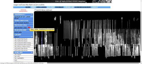
Once you’ve found the strip you’re interested in, click on it and you’ll get something like the page below left:
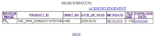
You’ll find it useful to click on the magnifying glass below ‘Browse Image’, as this will give you a thumbnail view of the strip you’ve selected. Bear in mind that the image may be upside down or inverted, depending on the direction of travel of the probe when it took the image.

When you’re happy you have the right one, click the ‘Download’ link and then go and do something useful with your time while the image downloads -
The next step is to get hold of the image software, which you can find on the Downloads page as the ‘SOFTWARE: PDS VIEWER’ link. You may find that the shortcut it installs doesn’t work, so browse to the folder in which you installed the software and run the ‘CH1_PDSViewer_Ver_1.1.jar’ file. Once installed and opened, you’ll see this screen (below left), which you need to click on to open the screen shown below right. Ignore any error messages it may give you about being unable to create data.
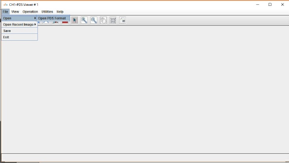
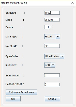
As shown in the screenshot, go to ‘File’, ‘Open PDS Image’ and browse to the file you downloaded and extracted. Look through the ‘DATA’ folder tree to find the .LBL file, select it and click ‘Open’. You’ll get a dialogue like this -
It will now import the image and calculate Min-
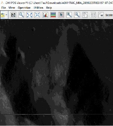
Here’s what you should get:
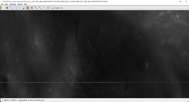
Unless this just happens to be the part of the image you need to be in, it’s not much use to you, so the best thing to do is to click the ‘Fixed Zoom Out’ tool to give a better overview, and then pan around to get what you want:
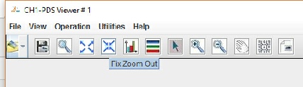
The software is clunky and may take time to respond to your demands to zoom around what has become a 5 Gb image with a 5 Gb temporary file behind it.
The best thing is not to be too precise, just get to roughly the right area and go to the ‘File’, ‘Save’ menu.
You’ll see a menu with lots of options. By all means explore all of them, but here’s what works for me.
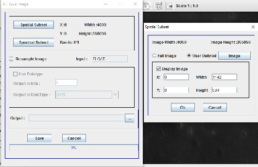
Click on ‘Spatial Subset’ -
Click OK’ when you’re done, then go to the ‘Output’ line. Browse to where you want to save the file, give it a name, then click ‘Save’.
If the software decides to throw a wobbly, you’ll need to close it down. Click on both the main software window and the smaller icon. When you click on the latter you’ll see this message:
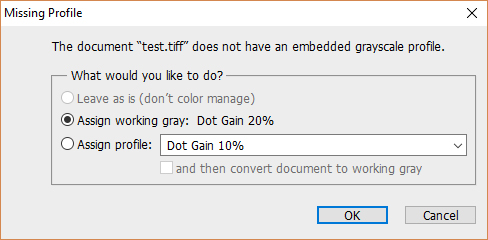
Just go with the default and click ‘OK’. Now we need to do something to work with the image. The way to turn it into something useful is to go to the HDR toning option and play around with the sliders that come up:
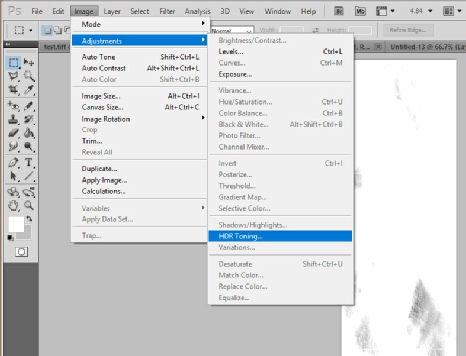
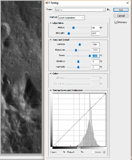
Just opening up the HDR menu will reveal the image, and the thing to do now is to play around with the sliders to enhance the image. I tend to push the detail right up and just tweak the others.
Once you’re done you might want to try increasing the dpi, sharpen, and do any other enhancing tricks you might know.
When you’re done, save the image and away you go, done!
As with other planetary data you can also open up the original downloaded image in QGIS. The knack here is to drag the ‘.LBL’ file into the layers window.
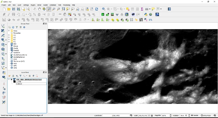
It’s much easier to move around, and as with other probe data you can export the frame as an image, but again as with other probes the quality isn’t as good.
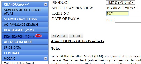
We can also use QGIS to play with the DEM data and get a 3D image, but to do that you’ll need to download a different set of images. First you’ll need to know which DEM data to get, and to do that you need to go back to the TMC mosaic’ and identify the strip you want to get a 3D for. The key information in there is the orbit on which the image was taken. When you have that, go to the DEM 10m search option and enter it in the box provided. Some areas aren’t covered by the 10m search, but are by the 25m one, so if at first you don’t succeed!
This will give you a result page like this:
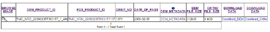
Download both the DEM and Ortho.
Once you’ve got them. the next step is to bring them both into QGIS by dragging them into the layers pane. You might want to go look at the page I wrote for JAXA data to cover how the next bits work in more detail.
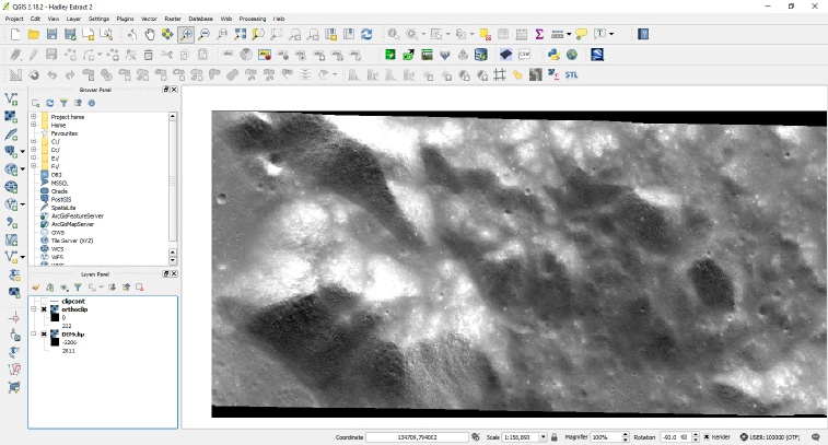
The key to getting a 3D rendering of this scene using the Qgis2gthreejs plugin is getting the coordinate system to work.
I have found a method that works some of the time -
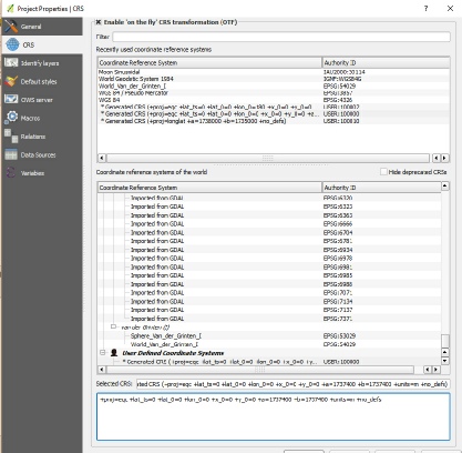
Tick the button that allows ‘On the fly’ CRS transformation at the top.
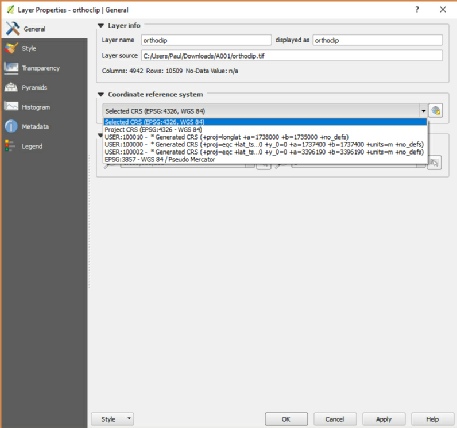
Now go to the the DEM and Ortho layers in turn.
Double click on the layer to get its properties dialogue box to appear. In the ‘General’ part, choose a CRS (see below left). The default one seems to work for me.
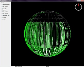
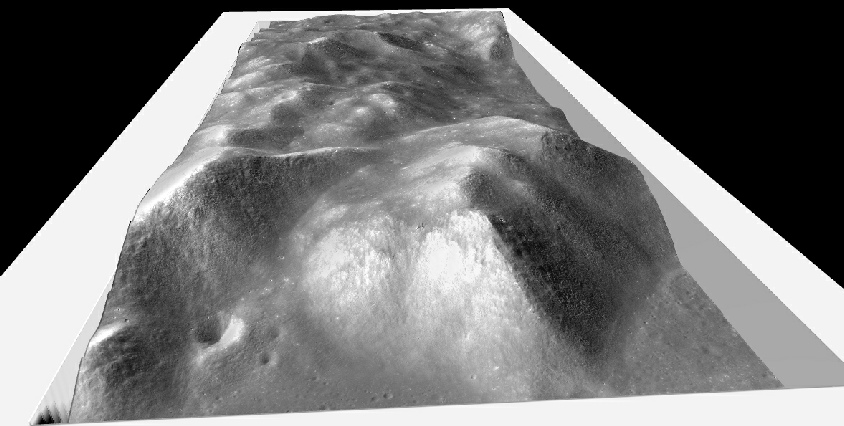
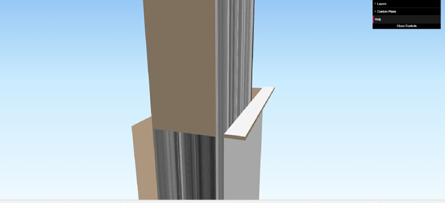
With any luck, when you run the Qgis2gthreejs plugin you’ll get a good 3D rendering. If not, it’ll look terrible and you’ll have to try again (see below).
Later versions of QGIS and the 3D plugin work slightly differently. See the JAXA page on this site for details.
Since this page was written, ISRO have begun (albeit very slowly) 3D data from their second lunar probe, Chandrayaan-
The data you need are here, and you;ll first need to register. You’ll also need a massive amount of patience to get the files, as the connection is extremely unreliable and doesn’t allow resuming when downloads fail.
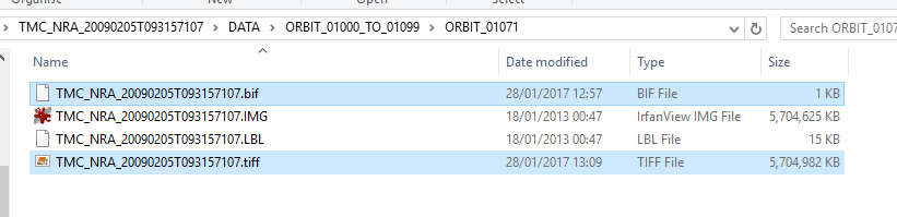
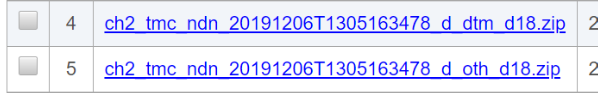
The files you need for 3D modelling are the orthographic and DTM geotiffs, which have ‘oth’ and ‘dtm’ in the filename:
Just delete the BIF and TIFF files and the software will open cleanly next time round.
Now you can go look at the image. Sadly, you won’t get much joy out of that as it will just appear as a white image. The next step is to head for the image editing software of your choice -
On opening the file you’ll see this message:
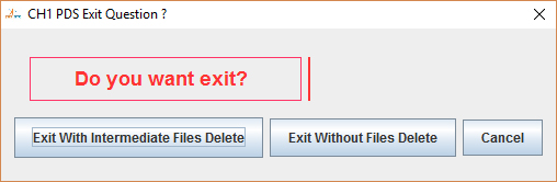
I’ve generally found it better to go for the option on the left ‘Exit with intermediate files delete’.
That said, it doesn’t always do that, so you may need to delete them yourself. In the example below the folder should only contain an LBL and IMG file. The other two have been created by the software while it works.
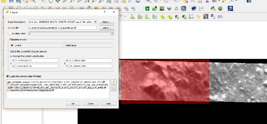
You could entire specific coordinates, or you could just click and drag a square on the layer itself as I’ve done above for the ortho layer.
Once it’s done, keep the dialogue box open and just change the source and destination layers so that you can do the DEM.
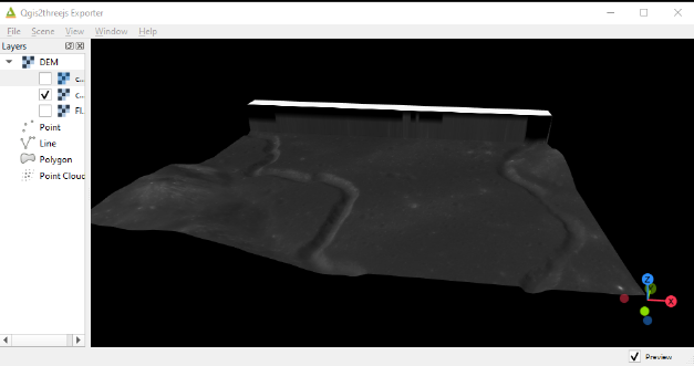
Here’s the image we’ve mostly been working on in this demonstration rendered in 3D. Click Close when you’re done (Clicking ‘OK’ will just repeat the process!’).
The key thing seems to be to get a coordinate system that is not in degrees as that throws out the calculations it has to make. The way to fix this is to reproject the coordinates so that everything involved in your QGIS project knows where everything is. Luckily this isn’t too difficult. First, go the Raster menu and open the ‘Projections’, ‘Warp (Reproject)’ sub-

You’ll now get a dialogue box asking you for various bits of information.
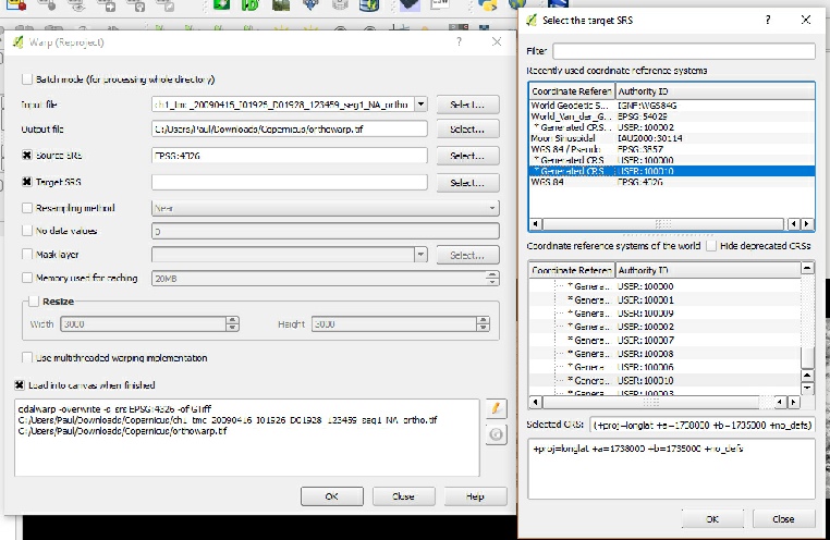
The first job is to pick the layer your re-
The Source SRS is the current coordinate system that is causing the problem in your source layer -
Click OK when you’ve done everything and it will process the information it’s been given and add a new layer with the correct coordinate reference. Repeat this for the other layer. If they don’t show immediately, right click on one of the new layers and choose ‘Zoom to layer’. You can safely remove the originals to keep things manageable. Your 3D projection should now work.
The other thing you can do to keep things manageable is reduce the image on screen to something more sensible -
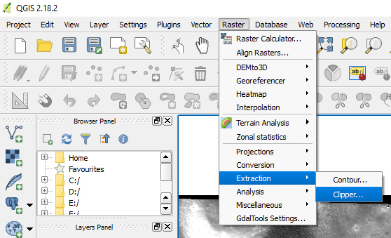
You’ll now get a dialogue box asking you where you want to save the new clipped layer, and how you want to select it.
As there are gaps in the data, you might find this useful to work out where you’re looking.
 Apollo Overview
3D Overview
Apollo Overview
3D Overview
To bring these into QGIS, all you need to do is drag the tiff images contained in those files into the software. One they’re in you can use the 3D plugin as before, but you will need to make an adjustment.
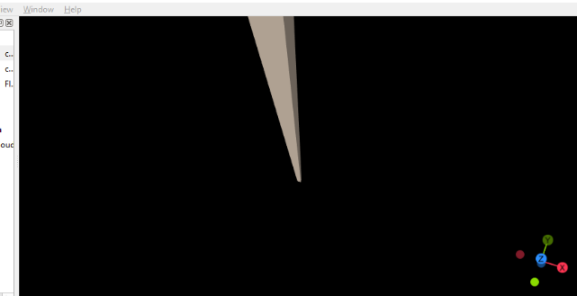
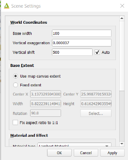
Because of the values the DTM models contain, the vertical height is exaggerated by a massive amount, like this:
To fix it, reduce the vertical exaggeration to about 0.000037:
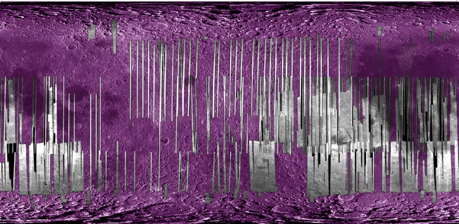
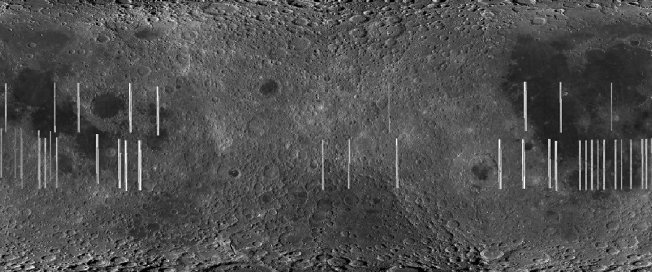
Data coverage is patchy so far, but hopefully will be increased soon. At the moment, this shows the TMC coverage we have:
The other files available for Chandrayaan-
You can open these in photoshop using the same method described above, but this time look for the width and height data:
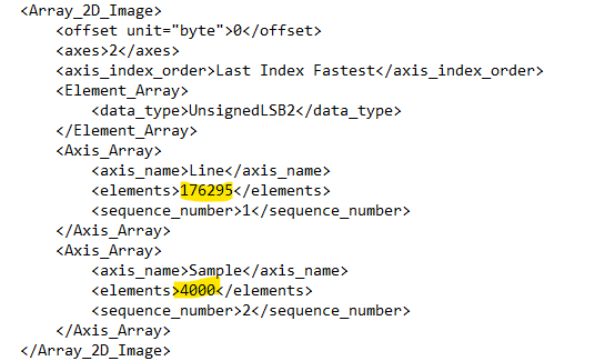
In this case the image is 4000 pixels wide and 176295 lines tall.
Have fun exploring India’s lunar data!